An Introduction to Big-O Notation

Measuring the efficiency of algorithms (in English and Japanese)

7 min readJan 29, 2021

When I first heard the word “algorithm” referenced in computer science as a 26 year old struggling to learn basic code, I dreaded the notion. “I should’ve paid more attention in high school math” and “If the engineers in my dad’s office struggle with this, there’s no hope for me” were a few of the self-defeating thoughts I had as I closed my laptop after a day of studying.

I believe for the majority of beginners like me who are getting their feet wet in programming, phrases such as “searching algorithms” or “time/space complexity” can seem quite intimidating and sow seeds of doubt in our own capabilities. Having said that, I think the concepts themselves aren’t difficult to grasp and well within reach of anyone who possesses a basic knowledge of numbers and logic.

This blog will serve mainly as a means to provide myself (and hopefully other struggling learners) a foundation to understand an algorithmic topic that will regularly present itself as the size and scale of our programs increase:

Big-O Notation.

Defining Big-O

Big-O notation is simply a way for programmers to talk about how efficient an algorithm is. An algorithm in programming is simply a procedure or method to solving a problem. How exactly do we measure efficiency in code? And why do we need a way to talk about it?

When we define a new method or function, there are often multiple implementations or ways to reach the same endpoint. Imagine a function where you take in a string input and return a new string with the characters reversed.

One common approach to this function

You might write and test this function, see that it works, and call it a day. But what about this implementation below?

Another approach using built-in Javascript methods

Or this one?

A third approach using recursion

If they all accomplish the same task, how do we come up with a system to determine which implementation is “best”? Do we measure how much time it takes to run each function on our computer? Is it the second one because it has the least lines of code? Why do we even care?

That’s where Big-O notation comes in. It gives us a way using precise vocabulary to talk about how our code performs and the trade-offs between different approaches. We should care about this because in certain situations such as debugging, it can help us understand and identify inefficiencies in our program.

How We Measure Big-O

To reference the suggestion from earlier, can we determine the efficiency of a program by how fast it runs? What if the computer I happen to be using is 15 years older than the latest MacBook Pro? Even if we had two computers of the same exact type and brand made in the same year, is there any guarantee the running times in seconds and milliseconds will be identical?

Instead of arbitrarily recording efficiency by counting in real time, Big-O notation counts the number of simple operations that the computer performs. On a general level, we can measure Big-O using what’s known as time complexity and space complexity.

We now have a look at a different function where we take in a number n, and return the sum of all integers from 1 to n inclusive.

Here we use a similar for loop to the first reverseString example

Let’s analyze this approach in terms of Big-O. Within the parameters of the for loop, we set a variable i and increment it on each cycle through. Inside the block, we perform an operation of adding i to sum each time until the middle parameter becomes false. Can we determine the total number of times these operations will occur when the function is called?

Yes! By the value of n.

Since our counter i starts at a value of 1 and increments by 1 every instance of the for loop, we can determine that the number of operations (and loops) will grow in proportion to n. This is an example of what we call time complexity in Big-O. In other words, the AddUpTo function has a Big-O time complexity of O(n). The bigger the value of n gets, the longer the function takes to run.

Here is a second solution to the same problem.

We no longer have to iterate through a loop, which means the number of operations we perform (one multiply *, one add +, one divide /) will remain constant regardless of how big a number gets passed in. As a result, the runtime is much more consistent compared to the first example, and we would consider this function to have a time complexity of O(1). This is also known as constant time.

Time Complexity and Space Complexity

Now we know that time complexity is the process of measuring the runtime of an algorithm based on the size of its input. On the other hand, space complexity measures how much additional memory we need to allocate in order to run the code in that algorithm. In short, how much space in memory do the contents of our function take up?

Below in this third example, let’s write a function where we accept an array of numbers and return the sum of them all.

We can deduce that sumArray has a Big-O time complexity of O(n) (n being the passed-in array). The more elements there are in arr, the more times we’ll have to pass through the loop, and the longer the runtime of sumArray becomes. However, the size of the input and the amount of loops this function performs does not play a part in calculating the space complexity (technically, when we calculate space in memory but exclude what’s taken up by the input, this is known as auxiliary space complexity).

In order to measure space complexity, we need to take a look at the primitives, strings, and other reference types located inside the function. Generally speaking, primitive values such as numbers, booleans, undefined, or null in Javascript have constant space O(1). Strings, arrays, and hashes have a space complexity of O(n), n in this case being the length of a string, the amount of elements in an array, or the number of key/value pairs in an object.

Let’s find all the variables and their value types that we declared in sumArray:

Notice how we are disregarding the input arr, which would have a space complexity of O(n). Because arr is not a variable within the function itself, we can conclude that sumArray runs with a time complexity of O(n) and a space complexity of O(1)! If we calculated a similar example where an array or object variable was declared INSIDE the function, that would’ve pushed our space complexity up to O(n).

The General Idea Behind Big-O

One important thing to remember about calculating the time and space complexity of our functions is that we care mostly about general trends. When all is said and done, Big-O is about “fuzzy counting”: identifying the efficiency of an algorithm through approximation rather than an exact calculation. As our variable n grows, what is the general trend in efficiency going to be?

Depending on the trend, our results could vary exponentially.

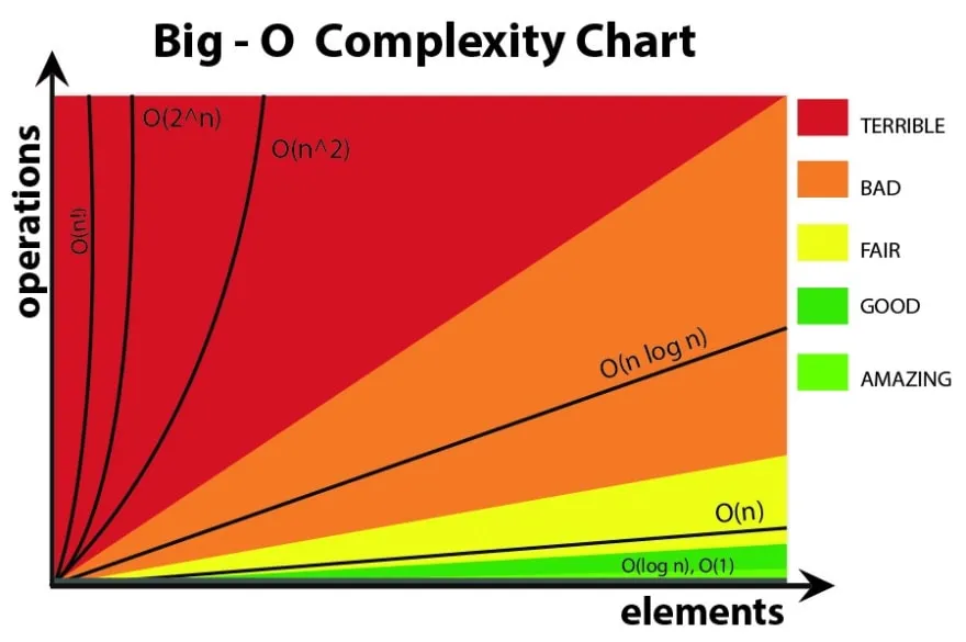
The most common complexities you’ll likely run into, from least-efficient to most, are:

O(n²)
O(n log n)
O(n)
O(log n)
O(1)

Big-O always refers to the worst case scenario for an algorithm. For example, let’s consider AddUpTo version #1 again.

If we passed in 1 as the value for n, our loop would only cycle through the block one time then return, allowing our function to achieve a constant run time. However, this would be considered as the best case scenario (also known as Ω(1)). As programmers, when we design a method or algorithm, our priority when it comes to analyzing efficiency should always be how our program performs given the least ideal conditions.

Calculating an algorithm’s Big-O is all about compromise. You may be able to create a function that runs on constant time O(1). However, let’s imagine your program will only work properly if the collection of data passed in is sorted. If that collection contained tens of thousands to hundreds of thousands of entries, what would be the Big-O required to sort through all the elements? What if the cumulative process becomes far more tedious than simply working with an unsorted collection? These are the types of questions that programmers continue to ask as they design and rework their programs.

Conclusion

With a solid grasp of the foundations of Big-O notation, many aspects of our code have the potential to be improved! On the other hand, it’s also important to remember that in many cases, it’s not about frantically searching for “better” more efficient solutions to a function. Neither is it about prioritizing Big-O of constant time complexity over other aspects of our code. It is merely an exercise in analyzing the performance of our programs through the general scope of time and space efficiency.

We are merely scratching the surface in regards to algorithms and data structures, but understanding Big-O notation will help open the door to all of these topics in the future!